patient_prognosis <-
  get_prognosis(gender = "Male",
                age = 45,
                comorbidities = c("diabetes", "hypertension")
)Introduction to R for
Health Data Science
Hands-on training
Language
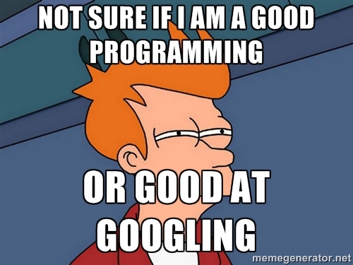
- What language do we use ?


How I have used R
- Public Health Medical Doctor @ Public Health Department
- Started using R during the COVID-19 pandemic
- Epicurves
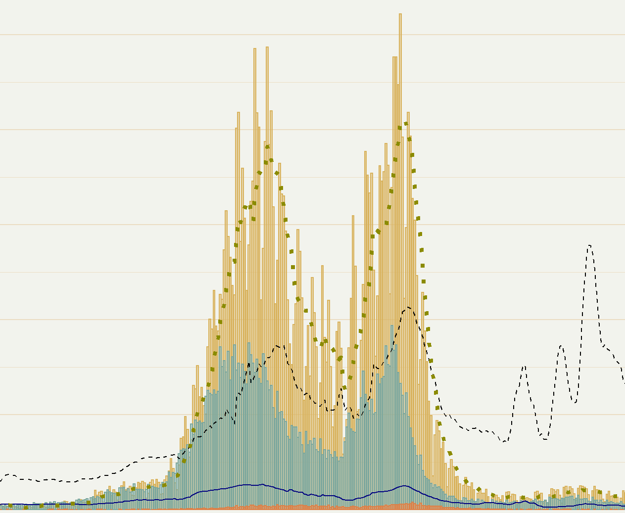
COVID-19 epicurve. Dates and counts are omitted for anonimity
How I have used R
- Public Health Medical Doctor @ Public Health Department
- Started using R during the COVID-19 pandemic
- Epicurves
- Forecasting
- Automating procedures
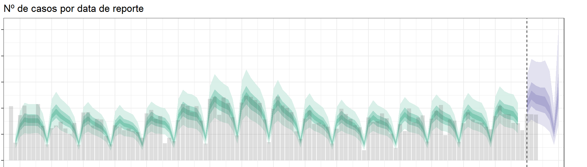
Covid case number forecasts by reporting date. Dates and counts are omitted for anonimity
How I have used R
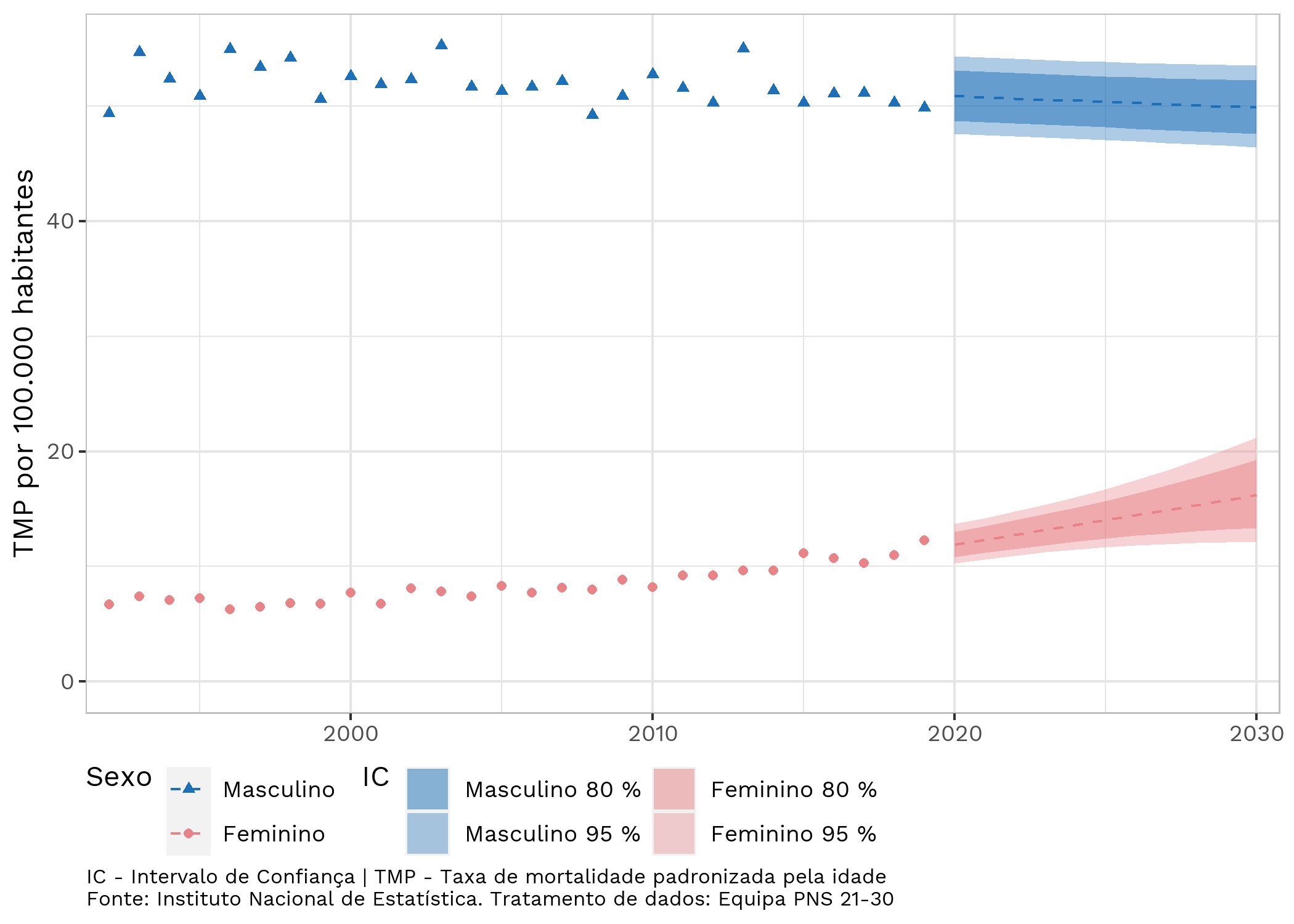
- Population health needs assessment of the Portuguese National Health Plan
- Mortality forecasting
How I have used R
- Population health needs assessment of the Portuguese National Health Plan
- Mortality forecasting
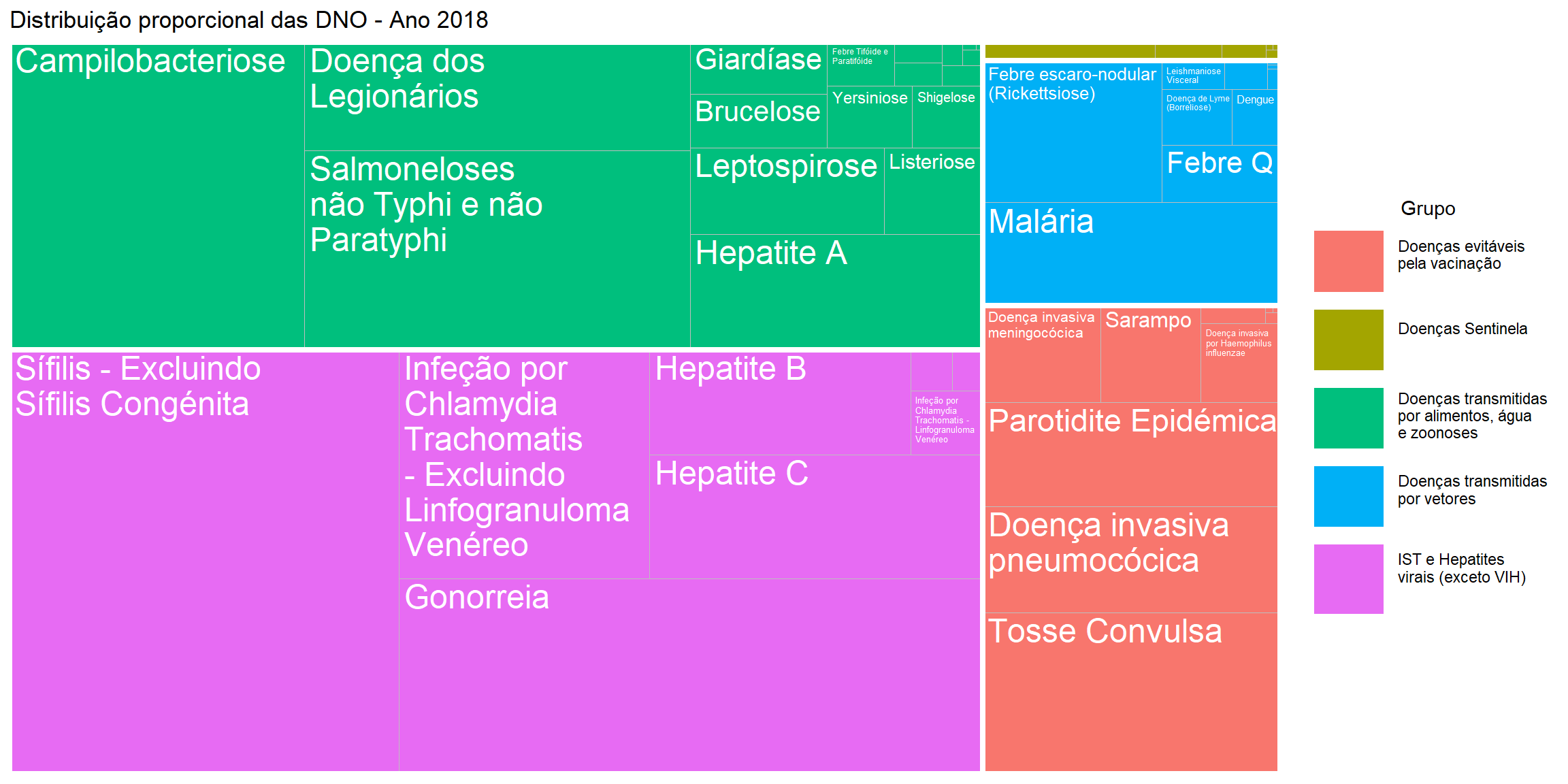
- Notifiable diseases
How I have used R
- Population health needs assessment of the Portuguese National Health Plan
- Mortality forecasting
- Notifiable diseases
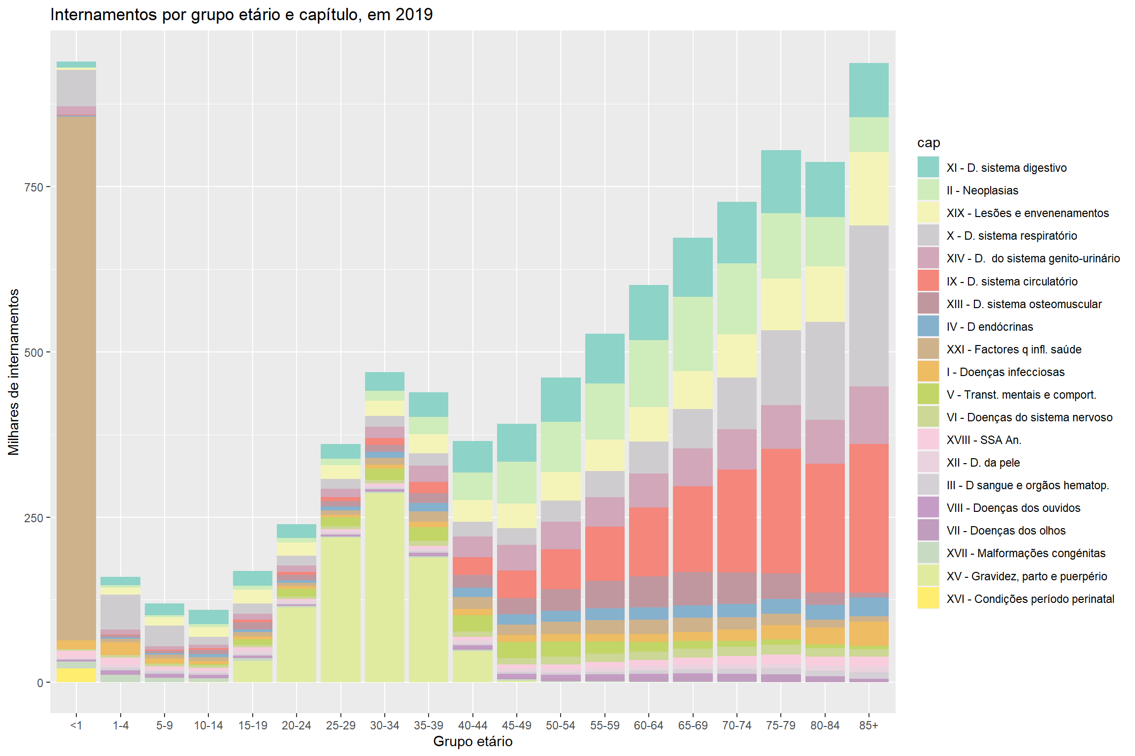
- Hospital morbidity
How I have used R
- Data analysis
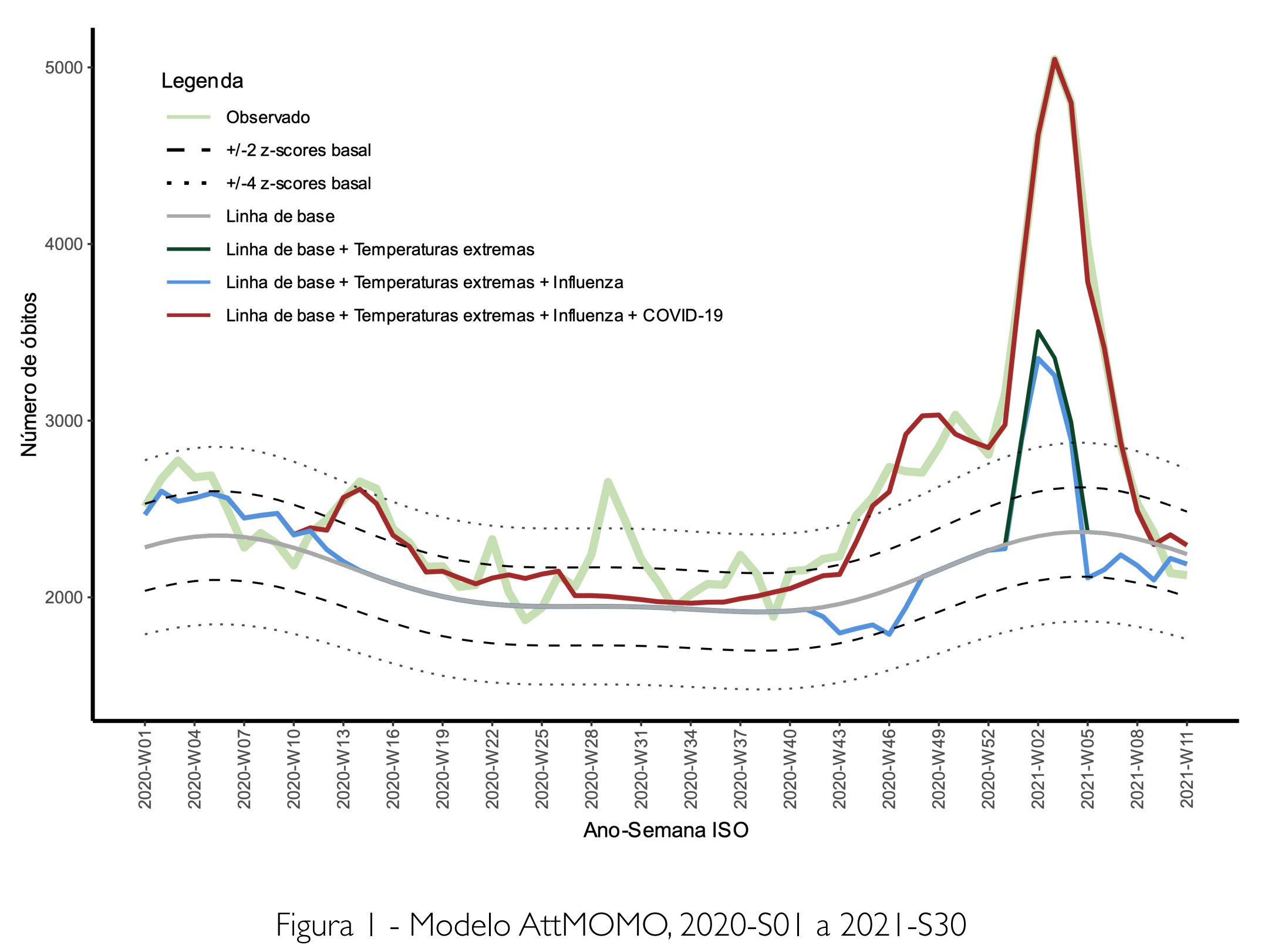
- Deaths attributable to Covid, Influenza and extreme temperatures
How I have used R
- Data analysis
- Deaths attributable to Covid, Influenza and extreme temperatures
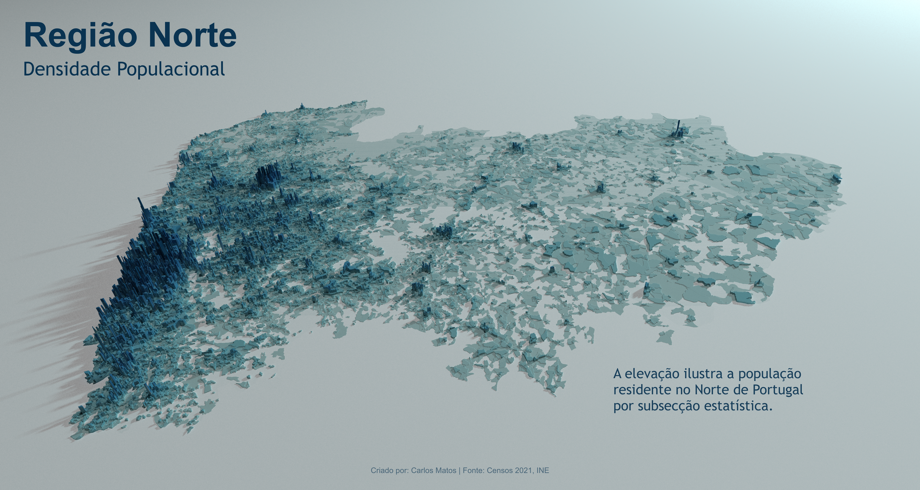
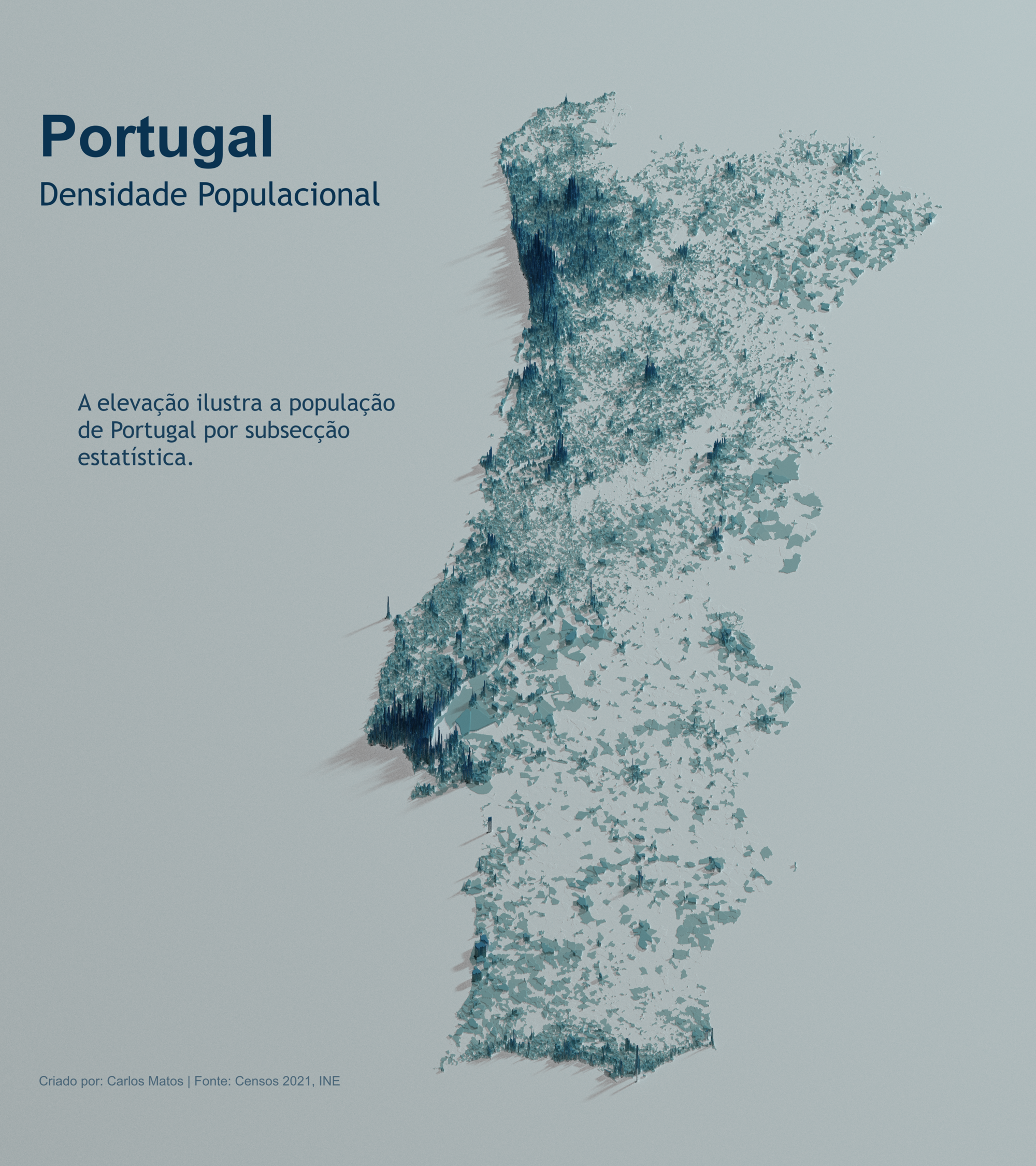
- Developed the ineptR package to facilitate and automate data extraction from Statistics Portugal with R
![]()

How I have used R
- Now working on improving dataviz skills and portfolio…
Goals for this course
- Be a learning catalyst
- Know what R is capable of
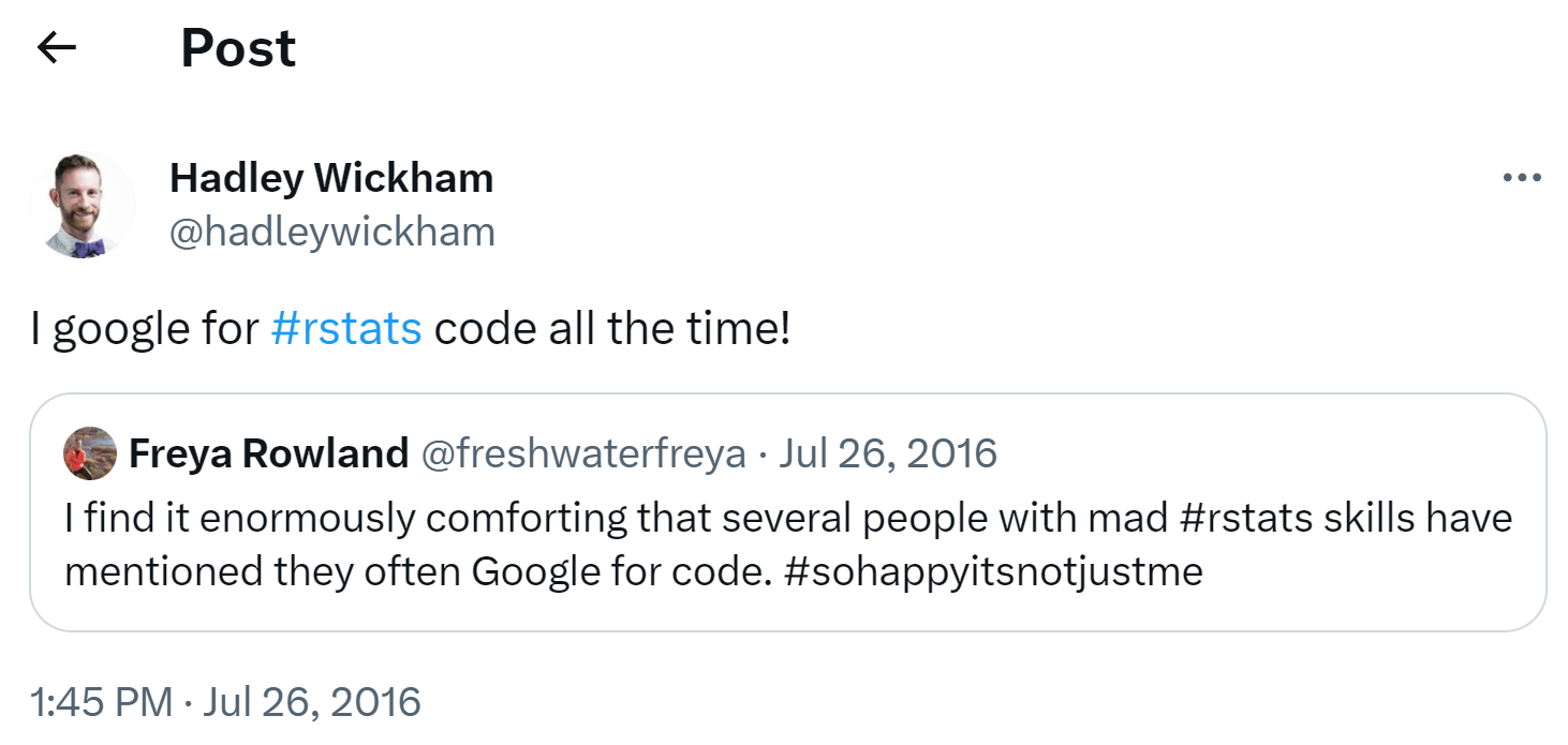
- Learn how to search the web for answers
- Gain a solid understanding of data wrangling with the tidyverse
- Learn the syntax of statistical models in R
- Be empowered to create and edit charts with ggplot
Goals for this course
- Communicate your results
- Static reports
- Dynamic dashboards
- Reproducible research and collaboration with version control
- A first step in the migration from other software!
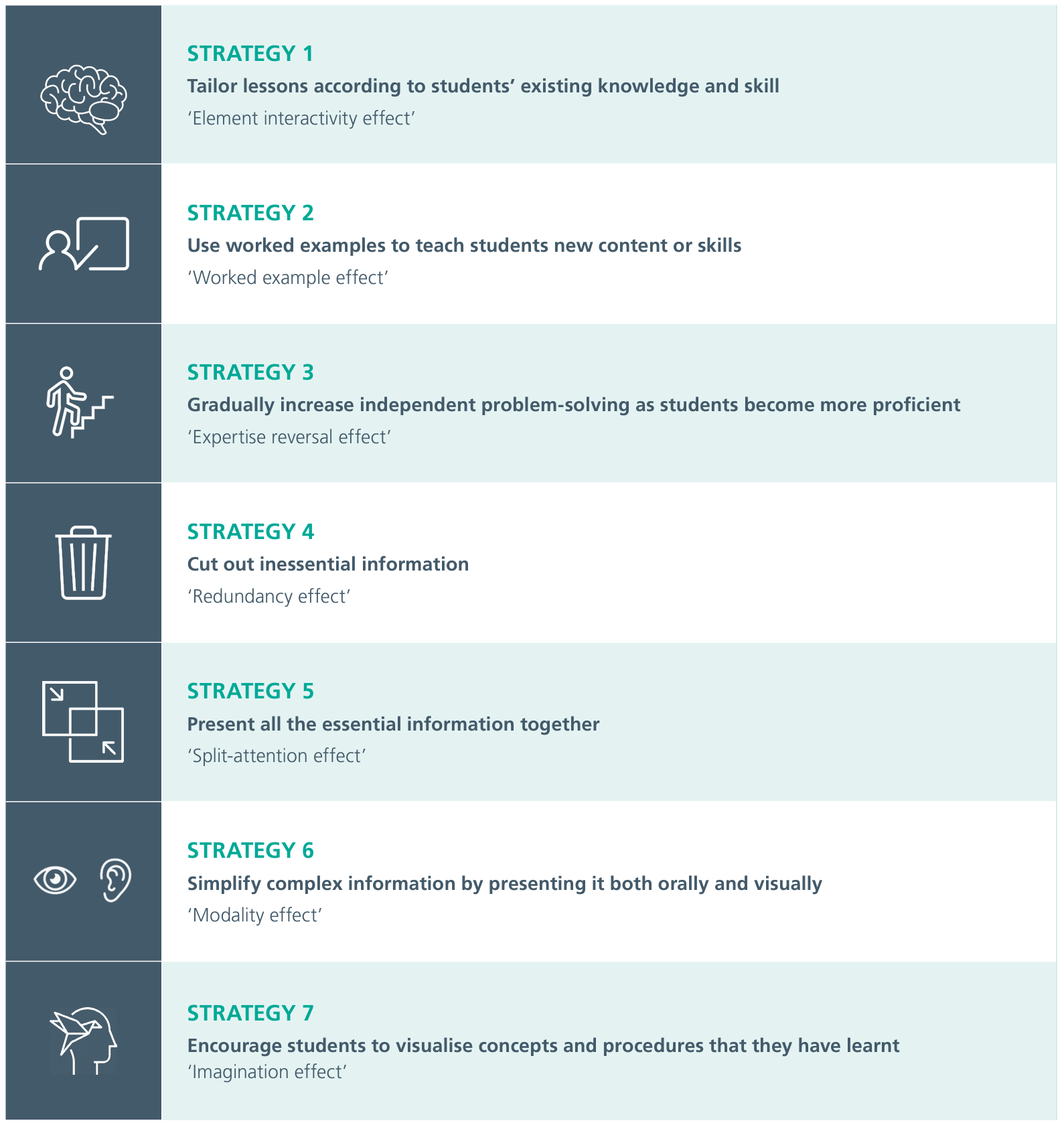
Methods
- Many worked examples
- Assuming no prior knowledge
- Start simple and increasing complexity over time
- Minimize redundancy
- R has many ways to achieve the same results. Choose one and stick to it.
Before we go into R…
Before we go into R…
R and RStudio
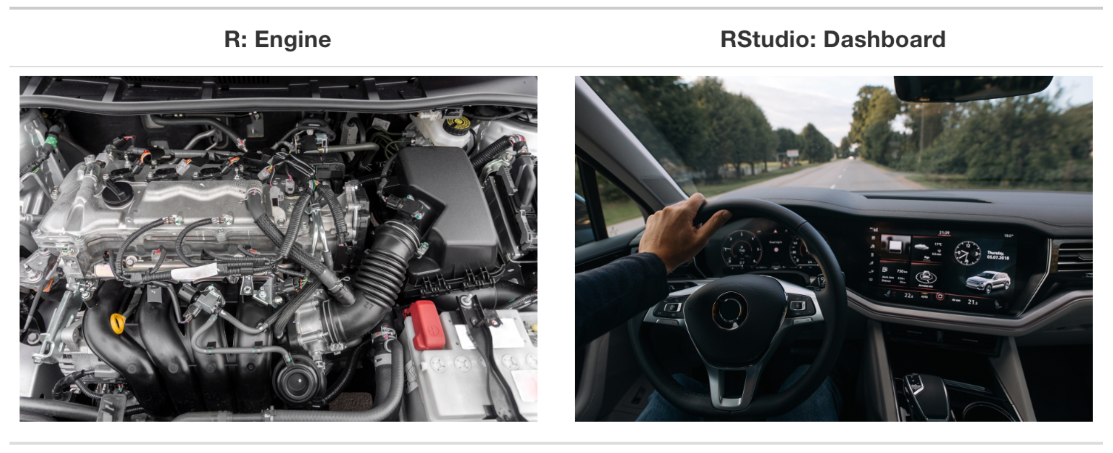
R vs RStudio
RStudio
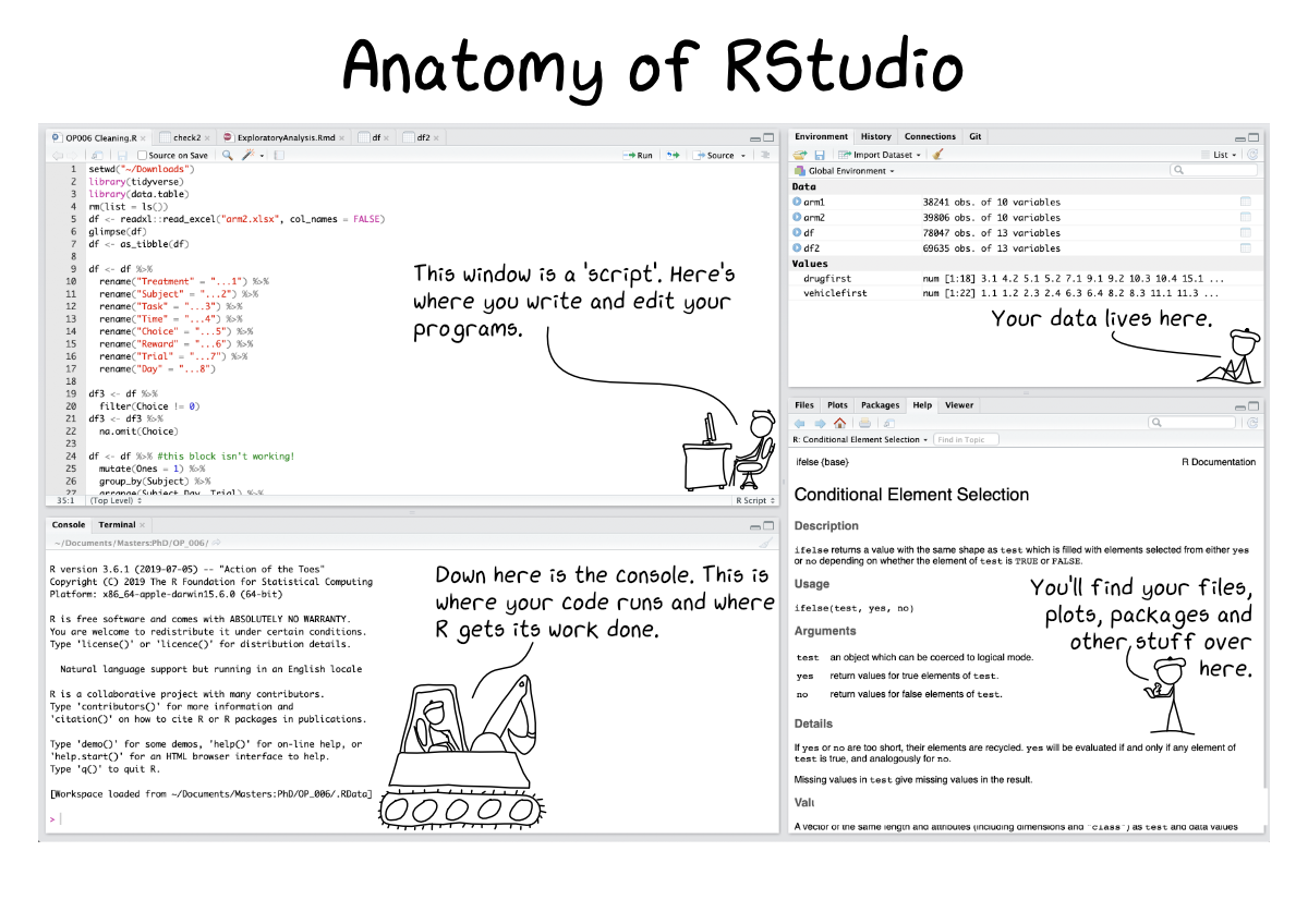
Anatomy of RStudio
Good vs bad code
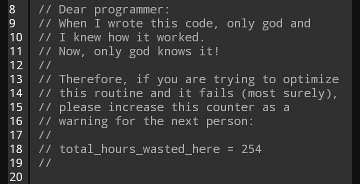
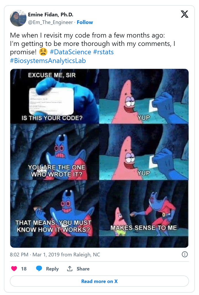
The single most important thing to remember
COMMENT YOUR CODE!
Key concepts

R vs R Packages
Objects - Everything we store in R. Can be variables, datasets, graphs, etc. Objetcs are assigned a name, which can be referenced in later commands
Functions - A function is a code operation that accept inputs and returns a transformed output. Read more in the Functions section. The basic unit of a package.
Packages - A bundle of functions that can be shared.
Scripts - A document/file that stores a set of commands.
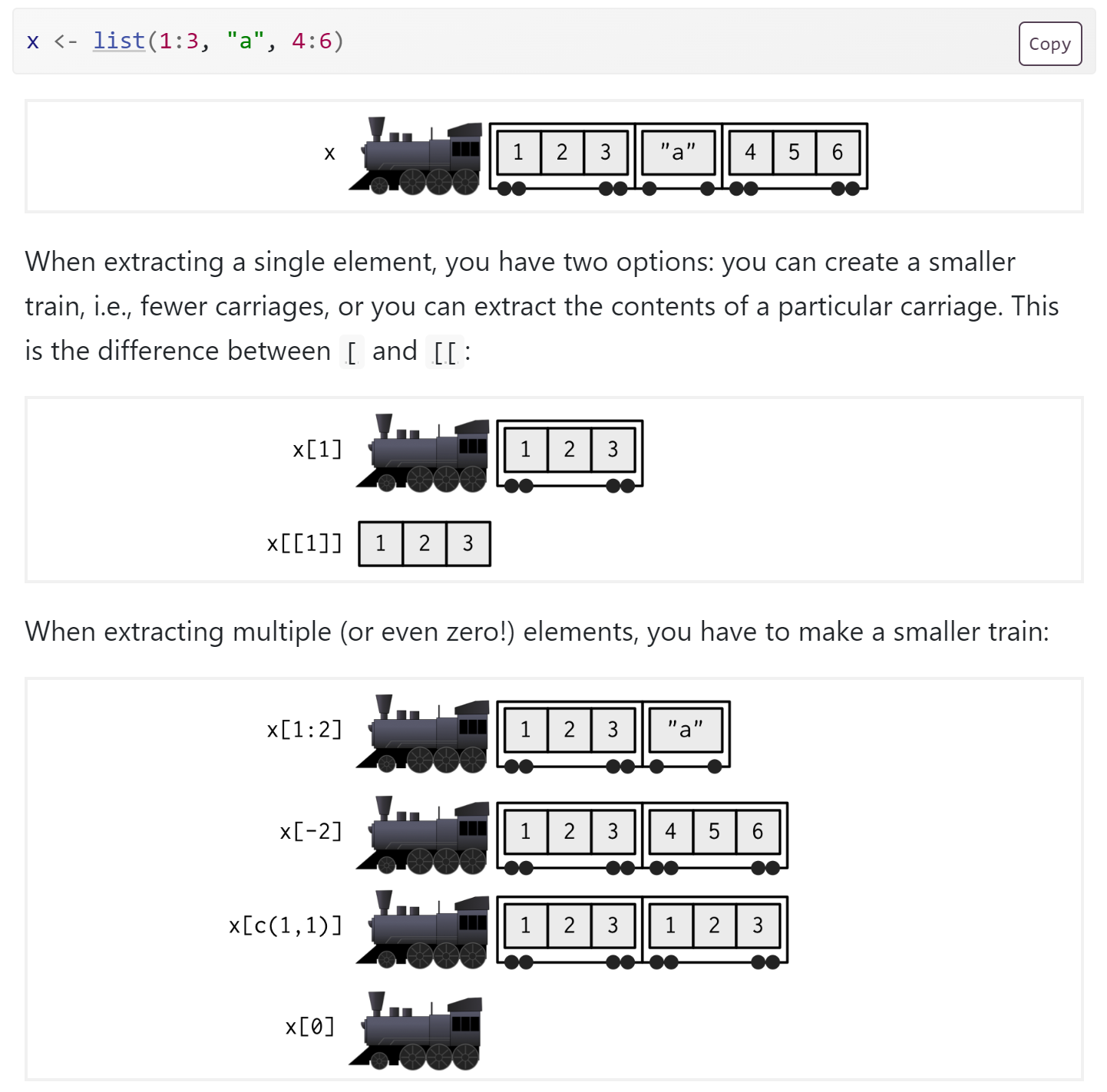
Exploring lists
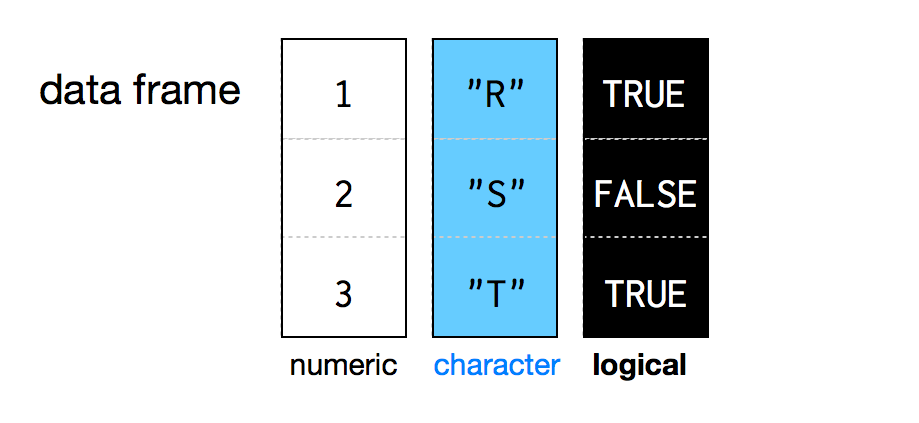
Data frames
- A 2D object (aka, a table…)
- You can think of it as a more rigorous Excel spreadsheet
- Unquestionably the most useful storage structure for data analysis
- Each column/variable is a vector
- Each column ALWAYS has the same type (contrary to Excel, where errors may occur)